This article develops a simple analytical model to measure the effects of inflation on the purchasing power of workers whose nominal wages remain unchanged. The analysis adopts a consumption-based perspective: households are assumed to preserve a constant level of real consumption for as long as their available financial resources permit.
No utility function is introduced. Instead, the household maintains a fixed quantity of real consumption, while the nominal cost of that consumption increases with the price level. Savings therefore operate as a residual component of the household budget, absorbing the loss of purchasing power caused by inflation.
Nominal wages and the interest rate paid on savings are assumed to remain constant throughout the period under consideration. Prices, by contrast, increase according to an exogenously determined annual inflation rate. The entire analysis is conducted using normalized monetary values.
The model is intended to describe short- to medium-term dynamics, during which nominal wages and deposit rates may not immediately adjust to changes in inflation. This assumption is particularly plausible when inflation is unexpected. Although the assumption becomes less realistic over longer periods, the model remains useful for illustrating the transitional burden imposed on workers by nominal wage rigidity.
Time is divided into discrete monthly periods indexed by \(t = 1,2,\ldots,T\).
The household receives a constant nominal wage \(w\). At the beginning of each period, it also has access to the savings accumulated during the preceding period, including the interest credited on those savings.
The household budget constraint is therefore:
\[ w + (1+r_0)S_{t-1} = C_t + S_t, \tag{1} \]
where:
Initial savings are assumed to be zero:
\[ S_0 = 0. \tag{2} \]
The household seeks to preserve a constant quantity of real consumption. Nominal consumption expenditure consequently varies with the price level:
\[ C_t = cP_t, \tag{3} \]
where \(c \in (0,1)\) represents the normalized level of real consumption and \(P_t\) is the price level of a representative consumption basket.
At the initial price level, \(c\) may also be interpreted as the proportion of the normalized wage devoted to consumption. The remaining share, \(1-c\), is potentially available for saving.
Let \(z_y\) denote the annual inflation rate. The equivalent monthly inflation rate \(z\) is given by:
\[ 1+z = (1+z_y)^{1/12}, \tag{4} \]
or equivalently:
\[ z = (1+z_y)^{1/12}-1. \]
If the initial price level is \(P_0\), the price level at time \(t\) is:
\[ P_t = P_0(1+z)^t. \tag{5} \]
For convenience, both the initial price level and the nominal wage are normalized:
\[ P_0 = 1 \qquad \text{and} \qquad w = 1. \tag{6} \]
Substituting Equations (3), (5), and (6) into the household budget constraint gives:
\[ 1 + (1+r_0)S_{t-1} = c(1+z)^t + S_t. \tag{7} \]
The corresponding law of motion for savings is:
\[ S_t = 1 + (1+r_0)S_{t-1} - c(1+z)^t. \tag{8} \]
Equation (8) describes the development of household savings when the nominal wage, the interest rate, and real consumption remain constant while prices increase.
Real consumption is fixed by assumption. Savings are therefore the residual component of the household budget and absorb changes in the nominal cost of maintaining that consumption.
The numerical simulation uses the following parameter values:
| Parameter | Value |
|---|---|
| \(r_0\) | \(0.0008\) |
| \(z_{y,1}\) | \(0.02\) |
| \(z_{y,2}\) | \(0.05\) |
| \(z_{y,3}\) | \(0.10\) |
| \(c\) | \(0.90\) |
| \(T\) | \(36\) |
The three annual inflation rates represent low, moderate, and high-inflation scenarios. The real consumption parameter is set equal to \(0.90\), meaning that the household initially devotes 90% of its monthly wage to consumption.
This assumption may be approximately representative of a household with a relatively high consumption-to-income ratio. Lower-income households would generally be expected to devote an even larger share of their income to consumption, whereas higher-income households may have a lower consumption share.
The monthly interest rate is approximately equivalent to a net annual deposit rate of 1%. It is held constant under all three inflation scenarios. This assumption represents a situation in which deposit rates adjust only slowly to inflation, particularly when the increase in inflation is unexpected.
The simulation covers 36 months. This period is sufficiently long to illustrate the cumulative effects of inflation while remaining short enough for nominal wage rigidity to be plausible.
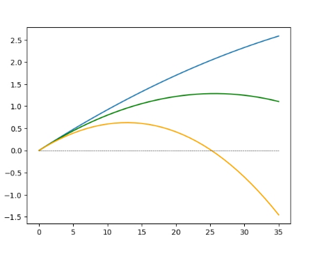
In each scenario, savings initially increase because the nominal wage exceeds current consumption expenditure. As prices continue to rise, however, the amount available for new savings declines. Savings eventually reach a maximum and subsequently begin to decrease.
Under high inflation, the household exhausts its savings within the 36-month period. Once savings are exhausted, the household can no longer maintain its assumed level of real consumption without borrowing, reducing consumption, increasing working hours, or obtaining a higher nominal wage.
The result can be summarized as follows:
Proposition 1. Given a constant nominal wage, a constant deposit rate, and a fixed level of real consumption, sufficiently high inflation exhausts household savings within a finite period.
Under the low- and moderate-inflation scenarios, savings may also eventually be exhausted. However, this occurs over a longer horizon, during which nominal wages, interest rates, or household behavior would be more likely to adjust.
The direct cost of inflation can be measured as the additional nominal expenditure required to purchase the same quantity of goods relative to the initial price level.
Let \(IC(t)\) denote the cumulative cost of inflation up to period \(t\):
\[ IC(t) = \sum_{i=1}^{t} \left(C_i-C_0\right). \tag{9} \]
Since \(C_i=cP_i\) and \(C_0=cP_0\), Equation (9) becomes:
\[ IC(t) = c\sum_{i=1}^{t} \left(P_i-P_0\right). \tag{10} \]
Using \(P_0=1\) and \(P_i=(1+z)^i\), we obtain:
\[ IC(t) = c\sum_{i=1}^{t} \left[(1+z)^i-1\right]. \tag{11} \]
The first component of Equation (11) is a finite geometric series:
\[ \sum_{i=1}^{t}(1+z)^i = \frac{(1+z)\left[(1+z)^t-1\right]}{z}. \tag{12} \]
The cumulative cost of inflation can therefore be written as:
\[ IC(t) = c \left[ \frac{(1+z)\left[(1+z)^t-1\right]}{z} -t \right]. \tag{13} \]
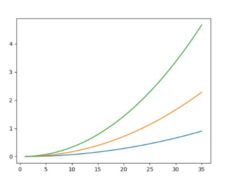
The cumulative cost increases nonlinearly under all three scenarios. The rate of increase is substantially greater when inflation is high because each increase in the price level becomes part of the base upon which subsequent price increases are calculated.
Since the monthly nominal wage has been normalized to one, \(IC(t)\) is expressed in monthly-wage units. This makes it possible to translate the cost of inflation into an equivalent number of working hours.
Assume that one monthly wage corresponds to 160 hours of work. The normalized hourly wage is then:
\[ w_h = \frac{w}{160} = \frac{1}{160}. \tag{14} \]
The cumulative cost of inflation expressed in working hours is:
\[ IC_h(t) = \frac{IC(t)}{w_h} = 160IC(t). \tag{15} \]
This measure indicates the number of additional hours that would have to be worked at the original hourly wage to compensate for the cumulative increase in consumption expenditure.
After 12 months, the cumulative costs rounded to the nearest working hour are:
\[ IC_{h,1}(12) \approx 19 \text{ hours}, \]
\[ IC_{h,2}(12) \approx 46 \text{ hours}, \]
\[ IC_{h,3}(12) \approx 92 \text{ hours}. \]
The result can be summarized as follows:
Proposition 2. Given a constant nominal hourly wage, maintaining the same level of real consumption during the first year requires the equivalent of approximately 19 additional working hours under 2% annual inflation, 46 hours under 5% inflation, and 92 hours under 10% inflation.
After 36 months, the cumulative costs are:
\[ IC_{h,1}(36) \approx 161 \text{ hours}, \]
\[ IC_{h,2}(36) \approx 410 \text{ hours}, \]
\[ IC_{h,3}(36) \approx 841 \text{ hours}. \]
At 160 working hours per month, 841 hours correspond to approximately:
\[ \frac{841}{160} \approx 5.26 \text{ months of work}. \tag{16} \]
Thus, under the high-inflation scenario, the cumulative increase in consumption expenditure over three years is equivalent to more than five months of work at the original hourly wage.
This does not mean that an employee could necessarily perform five additional months of overtime. Rather, the calculation expresses the purchasing-power loss in an intuitive and unit-independent form.
The real value of the constant nominal wage at time \(t\), relative to its initial value, is:
\[ w_t^{r} = \frac{w}{P_t}. \tag{17} \]
Given \(w=1\), \(P_0=1\), and \(P_t=(1+z)^t\), the proportional change in the real wage is:
\[ \Delta w_t^{r} = \frac{1}{(1+z)^t}-1. \tag{18} \]
After 36 months, the real wage declines by approximately:
\[ \Delta w_{1}^{r}(36) \approx -5.8\%, \]
\[ \Delta w_{2}^{r}(36) \approx -13.6\%, \]
\[ \Delta w_{3}^{r}(36) \approx -24.9\%. \]
These figures represent the loss of purchasing power of the nominal wage at the end of the period. They should be distinguished from the cumulative cost measure \(IC(t)\), which adds together the additional consumption expenditure incurred during every month of the period.
The model deliberately simplifies household behavior and the adjustment mechanisms operating in the economy.
First, nominal wages are assumed to remain constant. In practice, wages may be renegotiated, indexed, or adjusted when workers change employment. The model is therefore most informative during the period preceding such an adjustment.
Second, the interest rate paid on savings is held constant. In reality, nominal interest rates may increase in response to inflation and monetary-policy decisions. However, deposit rates may adjust with a delay and may remain below the inflation rate.
Third, real consumption is assumed to remain constant. Actual households may substitute cheaper goods, reduce discretionary expenditure, borrow money, or alter their saving behavior.
Fourth, the price level follows a deterministic path. Actual inflation is uncertain and varies across time and consumption categories. Households with different expenditure structures may therefore experience different effective inflation rates.
Finally, the model does not include taxation, unemployment risk, debt, transaction costs, or income from financial assets other than deposit interest.
This article has developed a simple model for measuring the burden of inflation when nominal wages are rigid and households attempt to preserve a constant level of real consumption.
The model shows that inflation initially reduces the household's capacity to accumulate new savings and eventually causes previously accumulated savings to decline. If inflation is sufficiently high and nominal wages remain unchanged, savings are exhausted within a finite period.
Expressing the cumulative cost of inflation in working hours provides an intuitive representation of the burden imposed on employees. Under the assumptions of the model, 2% annual inflation produces a cumulative three-year cost equivalent to approximately 161 hours of work. At 5% inflation, the corresponding cost is approximately 410 hours, while at 10% inflation it reaches approximately 841 hours.
The burden is likely to be especially significant for lower-income households because they generally devote a larger proportion of their income to consumption and possess smaller financial buffers. Such households have less scope to absorb price increases through reduced saving.
The analysis may be extended by introducing wage adjustments, heterogeneous consumption patterns, progressive taxation, stochastic inflation, alternative interest-rate paths, or borrowing constraints. A broader macroeconomic extension could also examine the relationship between inflation, labor-market mobility, wage negotiations, and resignation rates.
From a distributional perspective, the framework may help illustrate how the burden of inflation differs across income groups and how these differences may influence economic expectations, political preferences, and voting behavior.